stanflow is currently under active development–breaking changes may be made without warning, until a proper release.
stanflow offers an integrated, mildly opinionated access to a Stan-based Bayesian Workflow (Gelman et al. 2020). Much like the famous tidyverse package, stanflow is a metapackage which installs and attaches relevant Stan R packages, serving as a one-stop-shop for Bayesian modelling. stanflow draws heavy inspiration from tidyverse, and reuses portions of its codebase–however, stanflow eschews tidyverse packages (i.e., purrr, dplyr, etc.) for base R whenever necessary.
Installation
You can install the development version of stanflow from GitHub with:
# install.packages("pak")
pak::pak("VisruthSK/stanflow")
Usage
Here, we load stanflow and decide to use cmdstanr as the backend for brms.
library(stanflow)
#> ── Attaching Stan processing packages ─────────────────── stanflow 0.0.0.9000 ──
#> ✔ bayesplot 1.15.0.9000     ✔ projpred  2.10.0
#> ✔ loo       2.9.0           ✔ shinystan 2.7.0
#> ✔ posterior 1.6.1
#> ── Available Stan interfaces ────────────────────────────── setup_interface() ──
#> • brms     2.23.0     • rstan    2.32.7
#> • cmdstanr 0.9.0      • rstanarm 2.32.2
#> ── Conflicts ─────────────────────────────────────────── stanflow_conflicts() ──
#> ✖ posterior::rhat() masks bayesplot::rhat()
#> ℹ Use the conflicted package (<http://conflicted.r-lib.org/>) to force all conflicts to become errors
setup_interface(
  interface = "brms",
  dev = FALSE,
  brms_backend = "cmdstanr",
  cores = 2,
  quiet = FALSE,
  force = FALSE,
  check_updates = TRUE
)
#> ℹ Adding cmdstanr to setup because `brms_backend = 'cmdstanr'`
#> ℹ Attaching brms...
#> ℹ Configured brms: set `options(mc.cores = 2)` and `options(brms.backend = 'cmdstanr')`
#> ℹ Attaching cmdstanr...
#> The C++ toolchain required for CmdStan is setup properly!
#> ℹ Found CmdStan v2.37.0 at 'C:/Users/visru/.cmdstan/cmdstan-2.37.0'
#> ! Update available: v2.37.0 -> v2.38.0
#> ℹ Skipping update in non-interactive mode (set `force = TRUE` to upgrade).
#> ✔ Setup complete. brms, cmdstanr  packages are attached; you do not need to run `library()`.
set.seed(0)
flow_check()
#> ── Attaching Stan processing packages ─────────────────── stanflow 0.0.0.9000 ──
#> ✔ bayesplot 1.15.0.9000     ✔ projpred  2.10.0
#> ✔ loo       2.9.0           ✔ shinystan 2.7.0
#> ✔ posterior 1.6.1
#> ── Available Stan interfaces ────────────────────────────── setup_interface() ──
#> ✔ brms     2.23.0     • rstan    2.32.7
#> ✔ cmdstanr 0.9.0      • rstanarm 2.32.2
#> ── Conflicts ─────────────────────────────────────────── stanflow_conflicts() ──
#> ✖ brms::ar()      masks stats::ar()
#> ✖ brms::do_call() masks projpred::do_call()
#> ✖ brms::rhat()    masks posterior::rhat(), bayesplot::rhat()
#> ℹ Use the conflicted package (<http://conflicted.r-lib.org/>) to force all conflicts to become errors
With the first two commands (note that the setup_interface() call is unnecessarily verbose), users have access to everything they need to fit and interrogate Bayesian models. Specifically, those two commands will load the core stanflow packages: bayesplot, loo, posterior, projpred and shinystan, as well as setup brms to use the cmdstanr backend with as many cores as are available on your machine. These package (inlcuding brms and cmdstanr) are all “library()d” as well, so we can proceed with our analysis immediately.
cmdstanr_example()
#>    variable   mean median   sd  mad     q5    q95 rhat ess_bulk ess_tail
#>  lp__       -65.94 -65.62 1.39 1.19 -68.67 -64.29 1.00     1996     2876
#>  alpha        0.38   0.37 0.21 0.22   0.03   0.74 1.00     4087     3110
#>  beta[1]     -0.67  -0.67 0.25 0.25  -1.09  -0.27 1.00     4516     2758
#>  beta[2]     -0.27  -0.26 0.22 0.22  -0.64   0.09 1.00     3520     3012
#>  beta[3]      0.67   0.66 0.27 0.27   0.24   1.12 1.00     4444     3098
#>  log_lik[1]  -0.51  -0.51 0.10 0.10  -0.68  -0.37 1.00     3705     3254
#>  log_lik[2]  -0.41  -0.39 0.15 0.14  -0.67  -0.20 1.00     4327     3192
#>  log_lik[3]  -0.50  -0.46 0.22 0.20  -0.91  -0.20 1.00     3433     2935
#>  log_lik[4]  -0.45  -0.43 0.15 0.15  -0.73  -0.24 1.00     3605     2931
#>  log_lik[5]  -1.18  -1.16 0.28 0.28  -1.67  -0.75 1.00     4895     3413
#>
#>  # showing 10 of 105 rows (change via 'max_rows' argument or 'cmdstanr_max_rows' option)

fit1 <- brm(
  count ~ zAge + zBase * Trt + (1 | patient),
  data = epilepsy,
  family = poisson(),
  silent = TRUE,
  refresh = 0
)
#> Start sampling
#> Running MCMC with 4 chains, at most 2 in parallel...
#>
#> Chain 2 finished in 7.0 seconds.
#> Chain 1 finished in 7.0 seconds.
#> Chain 3 finished in 7.0 seconds.
#> Chain 4 finished in 7.4 seconds.
#>
#> All 4 chains finished successfully.
#> Mean chain execution time: 7.1 seconds.
#> Total execution time: 14.7 seconds.
summary(fit1)
#>  Family: poisson
#>   Links: mu = log
#> Formula: count ~ zAge + zBase * Trt + (1 | patient)
#>    Data: epilepsy (Number of observations: 236)
#>   Draws: 4 chains, each with iter = 2000; warmup = 1000; thin = 1;
#>          total post-warmup draws = 4000
#>
#> Multilevel Hyperparameters:
#> ~patient (Number of levels: 59)
#>               Estimate Est.Error l-95% CI u-95% CI Rhat Bulk_ESS Tail_ESS
#> sd(Intercept)     0.58      0.07     0.46     0.74 1.01      751     1459
#>
#> Regression Coefficients:
#>            Estimate Est.Error l-95% CI u-95% CI Rhat Bulk_ESS Tail_ESS
#> Intercept      1.76      0.12     1.53     1.99 1.01      728     1469
#> zAge           0.09      0.08    -0.07     0.26 1.00      848     1597
#> zBase          0.70      0.12     0.46     0.94 1.00      816     1347
#> Trt1          -0.26      0.17    -0.57     0.07 1.00      714     1196
#> zBase:Trt1     0.05      0.17    -0.28     0.38 1.00      904     1528
#>
#> Draws were sampled using sample(hmc). For each parameter, Bulk_ESS
#> and Tail_ESS are effective sample size measures, and Rhat is the potential
#> scale reduction factor on split chains (at convergence, Rhat = 1).

plot(fit1, variable = c("b_Trt1", "b_zBase"))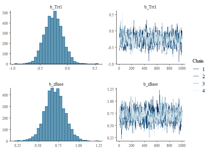
fit2 <- brm(
  count ~ zAge + zBase * Trt + (1 | patient) + (1 | obs),
  data = epilepsy,
  family = poisson(),
  silent = TRUE,
  refresh = 0
)
#> Start sampling
#> Running MCMC with 4 chains, at most 2 in parallel...
#>
#> Chain 1 finished in 11.3 seconds.
#> Chain 2 finished in 11.5 seconds.
#> Chain 4 finished in 13.6 seconds.
#> Chain 3 finished in 14.8 seconds.
#>
#> All 4 chains finished successfully.
#> Mean chain execution time: 12.8 seconds.
#> Total execution time: 26.3 seconds.
summary(fit2)
#>  Family: poisson
#>   Links: mu = log
#> Formula: count ~ zAge + zBase * Trt + (1 | patient) + (1 | obs)
#>    Data: epilepsy (Number of observations: 236)
#>   Draws: 4 chains, each with iter = 2000; warmup = 1000; thin = 1;
#>          total post-warmup draws = 4000
#>
#> Multilevel Hyperparameters:
#> ~obs (Number of levels: 236)
#>               Estimate Est.Error l-95% CI u-95% CI Rhat Bulk_ESS Tail_ESS
#> sd(Intercept)     0.37      0.04     0.29     0.46 1.00     1349     1967
#>
#> ~patient (Number of levels: 59)
#>               Estimate Est.Error l-95% CI u-95% CI Rhat Bulk_ESS Tail_ESS
#> sd(Intercept)     0.54      0.07     0.41     0.70 1.00     1125     1797
#>
#> Regression Coefficients:
#>            Estimate Est.Error l-95% CI u-95% CI Rhat Bulk_ESS Tail_ESS
#> Intercept      1.72      0.12     1.49     1.95 1.00     1088     2092
#> zAge           0.09      0.09    -0.09     0.26 1.00     1055     1569
#> zBase          0.70      0.12     0.47     0.94 1.00      971     1557
#> Trt1          -0.26      0.16    -0.59     0.06 1.00      922     1751
#> zBase:Trt1     0.06      0.16    -0.26     0.37 1.00     1045     1803
#>
#> Draws were sampled using sample(hmc). For each parameter, Bulk_ESS
#> and Tail_ESS are effective sample size measures, and Rhat is the potential
#> scale reduction factor on split chains (at convergence, Rhat = 1).

loo(fit1, fit2)
#> Warning: Found 6 observations with a pareto_k > 0.7 in model 'fit1'. We
#> recommend to set 'moment_match = TRUE' in order to perform moment matching for
#> problematic observations.
#> Warning: Found 58 observations with a pareto_k > 0.7 in model 'fit2'. We
#> recommend to set 'moment_match = TRUE' in order to perform moment matching for
#> problematic observations.
#> Output of model 'fit1':
#>
#> Computed from 4000 by 236 log-likelihood matrix.
#>
#>          Estimate   SE
#> elpd_loo   -671.9 36.8
#> p_loo        94.4 14.5
#> looic      1343.8 73.6
#> ------
#> MCSE of elpd_loo is NA.
#> MCSE and ESS estimates assume MCMC draws (r_eff in [0.4, 2.2]).
#>
#> Pareto k diagnostic values:
#>                          Count Pct.    Min. ESS
#> (-Inf, 0.7]   (good)     230   97.5%   142
#>    (0.7, 1]   (bad)        5    2.1%   <NA>
#>    (1, Inf)   (very bad)   1    0.4%   <NA>
#> See help('pareto-k-diagnostic') for details.
#>
#> Output of model 'fit2':
#>
#> Computed from 4000 by 236 log-likelihood matrix.
#>
#>          Estimate   SE
#> elpd_loo   -594.6 13.9
#> p_loo       107.2  7.1
#> looic      1189.1 27.7
#> ------
#> MCSE of elpd_loo is NA.
#> MCSE and ESS estimates assume MCMC draws (r_eff in [0.4, 1.7]).
#>
#> Pareto k diagnostic values:
#>                          Count Pct.    Min. ESS
#> (-Inf, 0.7]   (good)     178   75.4%   248
#>    (0.7, 1]   (bad)       55   23.3%   <NA>
#>    (1, Inf)   (very bad)   3    1.3%   <NA>
#> See help('pareto-k-diagnostic') for details.
#>
#> Model comparisons:
#>      elpd_diff se_diff
#> fit2   0.0       0.0
#> fit1 -77.3      27.4
Code snippets above are taken from the brms README but aren’t directly comparable.